Network Analysis

Goal & Objectives

The overall goal of this lab is to complete network analysis successfully.  This lab involved setting up a python script with variables, querying statements, loading modified features into the Network Analysis Window, calculating routes and closest facilities, and building a data flow model to calculate the closest facility route.  Finally, we had to calculate the cost of sand truck travel on roads by county.


Methods 

          The objectives for the first half of the lab consisted of setting up and running a python script (Figure 1).  I set up the script, imported the modules and environments and prepared the script. I then had to set up variables for the list of feature classes we were using.  Variables are used to substitute the actual name to make scripting easier.  I then wrote several SQL statements that together selected all mines that were within 1.5 km of a terminal and removed those mines.  

Figure 1

          The second part of the lab consisted of actual network analysis.  Refer to the data flow model below (Figure 2).  I added the streets network data set from ESRI and opened the network analyst window.  I first used Make Closest Facility Layer to add a closest facility layer from the network analyst menu.  After that I solved the layer and the routes were added.  I then had to add the desired locations for network analyst, both the facility and incident locations.  I proceeded to solve the layer, select and copy that data and project it in a state plane Wisconsin coordinate system in meters.  I then had to intersect Wisconsin county boundaries with the output of the project tool.  After the intersection I used Summary Statistics to summarize the newly intersected data.  The next step in this process was to find out how many miles each route was on a county level and the annual cost of that transportation.  I added two fields and calculated both fields.  The calculations for each field are below:

Miles Field:      [SUM_Shape_Length]/1609.34

Cost Field:        ([miles]*100) *.022

This brought me to my final table containing my two new fields, length in miles and cost in dollars.  

I put together two maps depicting the routes and cost after everything was completed.  

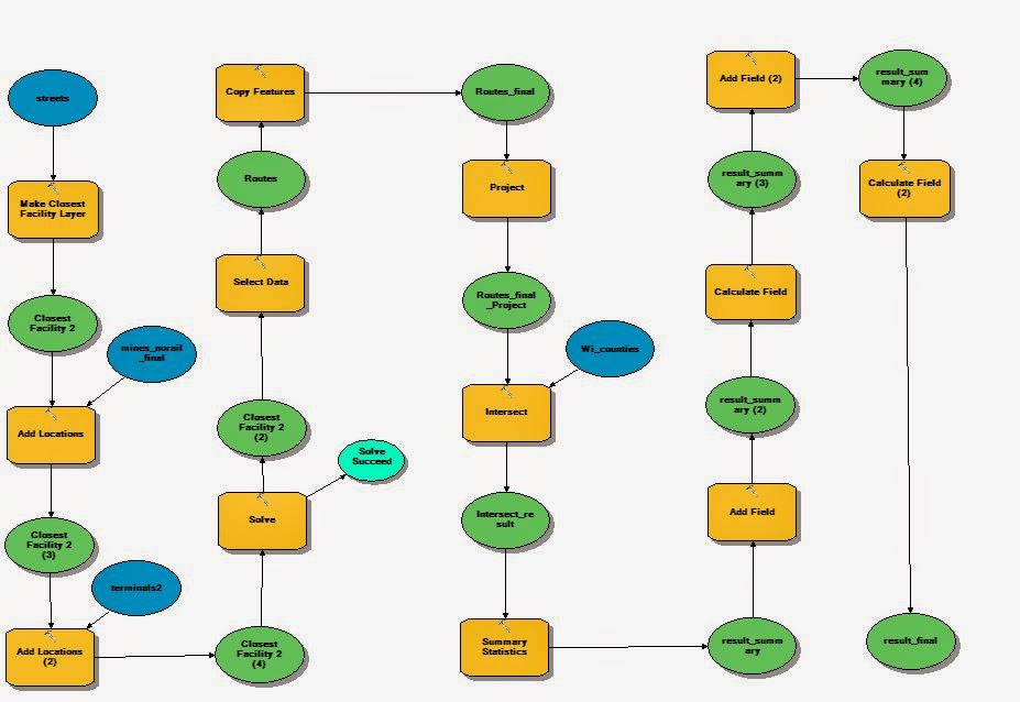
Figure 2
'

Results and Discussion

The results below include a network map of sand mines and terminal locations, a county map of annual cost of transportation, and the final table with the miles and cost fields.  It should be noted that all of the results here are hypothetical and do not relate to the real world.  In Figure 1 below, sand mines are being routed to closest facilities and several unused terminals.    

Figure 3

Figure 2 below shows the annual cost of transportation on a county level.  

Figure 4

Figure 3 shows the final table with the new calculated fields: miles and cost

Figure 5

Conclusion

Overall this lab was a very good introduction to the tools and processes involved with network analysis. This exercise used many different tools and forced us to use our geospatial problem solving skills.  The skills used in this lab are extremely practical to the real world and I now have a familiar background with network analysis. By creating a python script, and using that script to query and use data, we were able to create a new feature class and use that feature class for network analysis.  Network analysis is a vital tool in the geospatial world and I feel that this lab has provided me with the knowledge to complete network analysis on my own with real world problems.